Genome Spot

Counting the number of reads that align to certain genomic features is a key element of many next gen sequencing analysis pipelines. For RNA-seq, this is commonly used to count reads aligning to exons, while for ChIP-seq this is used to count reads over a promoter or other region of interest. There are several available tools for performing this task and in this post I will compare the three of the most commonly used: bedtools multicov htseq-count featureCounts I took one of the bam files from the recent RNA-seq series  of posts and subsampled it using samtools and shuf into file sizes of 1M, 2M, 5M, 10M reads, as well as the bam file containing 25.4M reads. I  then used the benchmarking script described in the previous post  to record execution time, CPU usage and peak memory for read counting to generate a gene-wise matrix. I used featureCounts in the single thread mode as well as the parallel mode (maximum of 8 cores). Execution time for read counting...

Bioinformaticians strive for accurate results, but when time or computational resources are limited, speed can be a factor too. This is especially true when dealing with the huge data sets coming off sequencers these days. When putting together an analysis pipeline, try taking a small fraction of the data and perform some benchmarking of the available tools. Benchmarking could be as simple as using time : time ./script1.sh time ./script2.sh But if you need a little more detail, this benchmarking approach captures peak memory usage and average CPU utilisation too. 1. Set up a list of commands/scripts in a file called "codes.txt" Here is a list of commands that I used in a previous post : $ cat codes.txt cat test.fastq > /dev/null zcat test.fastq.gz > /dev/null bzcat test.fastq.bz2 > /dev/null pigz -dc test.fastq.gz > /dev/null pbzip2 -dc test.fastq.bz2 > /dev/null plzip -dc test.fastq.lz > /dev/null 2. Setup the benchmarking script ...

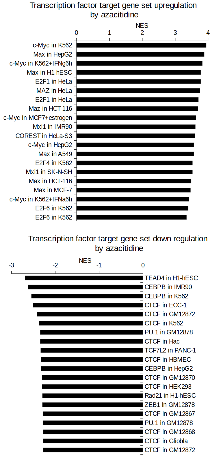
So far in this series of posts we've analysed the effect of azacitidine on AML3 cell gene expression using publicly available RNA-seq data. Our pathway analysis showed many interesting trends, but unravelling all the different mechanisms from this point can be really hard. In order to identify the major players at the chromatin level, it can be useful to integrate transcription factor binding data and see whether targets of a particular transcription factor are differentially regulated in a pathway analysis. The problem with this analysis in the past was that ChIP-seq datasets were in varying formats on GEO and processing these into a standardised format would be too time consuming. With the advent of the ENCODE Project , there is now a large body of transcription factor binding data in a uniform format ( link ), that is being mined in many creative ways. In our group, we used this approach extensively ( here , here and here ). In this post, we will mine ENCODE transcription f...

In our RNA-seq series so far we've performed differential analysis and generated some pretty graphs, showing thousands of differentially expressed genes after azacitidine treatment. In order to understand the biology underlying the differential gene expression profile, we need to perform pathway analysis. We use Gene Set Enrichment Analysis ( GSEA ) because it can detect pathway changes more sensitively and robustly than some methods. A 2013 paper compared a bunch of gene set analyses software with microarrays and is worth a look. Generate a rank file The rank file is a list of detected genes and a rank metric score. At the top of the list are genes with the "strongest" up-regulation, at the bottom of the list are the genes with the "strongest" down-regulation and the genes not changing are in the middle. The metric score I like to use is the sign of the fold change multiplied by the inverse of the p-value, although there may be better methods out there...

Next generation sequencing is driving genomics into realm of big data, and this will only continue as NGS moves into the hands of more and more researchers and clinicians. Genome sequence datasets are huge and place an immense demand on informatics infrastructure including disk space, memory and CPU usage. Bioinformaticians need to be aware of the performance of different compression software available to make the most out of their hardware. In this post, we'll test the performance of some compression algorithms in terms of their disk-saving ability as well as speed of decompression/compression. The file that we're working on is an RNA-seq fastq file that is 5.0 GB in size and contains 25.8 million sequence reads on 103.0 million lines. Here is the top 10 lines. @SRR1171523.1 Y40-ILLUMINA:15:FC:5:1:8493:1211 length=36 ACTTGCTGCTAATTAAAACCAACAATAGAACAGTGA +SRR1171523.1 Y40-ILLUMINA:15:FC:5:1:8493:1211 length=36 B55??4024/13425>;>>CDD@DBB<<<BB...

We will continue our  series  in the analysis of our azacitidine treated AML3 cell RNA-seq gene expression data set by generating a  multidimensional scaling plot . This is a potentially useful way of showing variability in datasets, especially when the number of samples is large. Trawling the blogs, I found a really quick and easy way to do this in R (thanks  Michael Dondrup@BioStars ) that can be used to analyse the count matrix. x<-scale(read.table("CountMatrix.xls", row.names=1, header=TRUE)) pdf("MDSplot.pdf")  plot(cmdscale(dist(t(x))), xlab="Coordinate 1", ylab="Coordinate 2", type = "n") ; text(cmdscale(dist(t(x))), labels=colnames(x), )  dev.off() Multidimensional scaling (MDS) plot for public gene expression data ( GSE55123 ).  The closer the labels are together, the more similar the samples are. So it is good to see that the untreated samples are clearly separated from the azacitidine treated samples. UNTR...

In the last post of this series , I left you with a gene expression profile of the effect of azacitidine on AML3 cells. I decided to use the DESeq output for downstream analysis. If we want to draw a heatmap at this stage, we might struggle because the output provided by the DEB applet  does not send back the normalised count data for each sample. It is not really useful to plot all 5704 genes with FDR adjusted p-values <0.05 on the heatmap, so I will simply show the top 100 by p-value. Here are the general steps I will use in my R script below: Read the count matrix and DESeq table into R and merge into one table Sort based on p-value with most significant genes on top Select the columns containing gene name and raw counts Scale the data per row Select the top 100 genes by significance Generate the heatmap with mostly default values Google  searches  show that R has some quite elaborate heatmap options, especially with features from ggplot2 and RCol...

So far in this RNA-seq analysis series of posts, we've done a whole bunch of primary analysis on GSE55125  and now we are at the stage where we can now perform a statistical analysis of the count matrix we generated in the last post  and look at the genes expression differences caused by Azacitidine. For this type of analysis we could load our data into R and perform the analysis ourselves, but for a simple experiment design with 2 sample groups in triplicate without batch effects or sample pairing I want to share with you an easy solution. DEB is a online service provided by the  Interdisciplinary Center for Biotechnology Research (ICBR) University of Florida that will analyse the count matrix for you with either DESeq, edgeR or baySeq. Their Bioinformation paper is also worth a look. As with all aspects of bioinformatics, format is critical. You need to follow the specified format exactly. Here is what the head of my count matrix looks like: gene UN...

In this RNA-seq analysis series of posts , we're going through an RNA-seq analysis workflow. So far, we've downloaded, done QC and aligned the reads. In this post, we will count the reads aligning to exons and generate a count matrix for statistical analysis. My overall strategy is to use bedtools to count reads over exons. To do that, I'll need a bed file containing all exons. I could use UCSC genes, but I'd rather use the latest Ensembl version. Create exon bed file  To begin, we need a list of known exons. I will use the latest Ensembl human gene annotation gtf file from their ftp server. Then extract the exon entries with grep and then rearrange the gene accession and symbol information into a temporary bed file. The temporary bed file is exploded on gene name and then overlapping exons are merged with bedtools. #!/bin/bash wget ftp://ftp.ensembl.org/pub/release-76/gtf/homo_sapiens/Homo_sapiens.GRCh38.76.gtf.gz zcat Homo_sapiens.GRCh38.76.gtf.gz \ | gr...

In this series of posts, we're going through an RNA-seq analysis workflow. So far, we've downloaded and inspected sequence quality . In this post, we will align the paired end data to the human genome with Tophat . Part 1 is to get a suitable reference genome sequence. I chose download the most recent human genome sequence from the Ensembl ftp site  (Homo_sapiens.GRCh38.dna_sm.primary_assembly.fa). axel --num-connections=6 ftp://ftp.ensembl.org/pub/release-76/fasta/homo_sapiens/dna/Homo_sapiens.GRCh38.dna_sm.primary_assembly.fa.gz Once downloaded, the genome needs to be uncompressed and indexed with bowtie2. This will take a few hours. REF=Homo_sapiens.GRCh38.dna_sm.primary_assembly.fa gunzip ${REF}.gz bowtie2-build $REF $REF Next step is to use Tophat to align the reads in paired-end mode. Tophat is smart enough to recognise the bz2 compression. The script also indexes the bam files and generates some familiar samtools statistics. #!/bin/bash REF=/path/to/gen...

In a previous post , we downloaded RNA-seq data from GEO ( GSE55123 ) . Lets continue with the processing of this data by performing QC analysis. In a previous post , I went into a bit more detail, but here we will simply use fastx_quality_stats from the fastx toolkit to have a look at quality scores among the data sets. The general strategy was to unzip the data on the fly, convert to tabular format and then select a random 1 million sequences and then submit these to fastx_quality_stats. So having a look through the output file, shows very high quality scores with median scores >36 which suggests this dataset is very high quality. Below see the code used and a graph of median quality scores throughout the run. #!/bin/bash for FQZ in *bz2 do echo $FQZ pbzip2 -dc $FQZ | paste - - - - | shuf | head -1000000 \ | tr '\t' '\n' | fastx_quality_stats | cut -f1,6-9 done | tee quality_analysis.txt Mean cycle base quality for GSE55123 RNA-seq data shows very h...

Here is a 1 line command to turn a list of sequences into a fasta file. $ cat seq.txt  CAACACCAGTCGATGGGCTGT CAACACCAGTCGATGGGCTGTC CAACACCAGTCGATGGGCCGT TAGCTTATCAGACTGATGTTGA TAGCTTATCAGACTGATGTTGAC We use nl to count the lines, then sed to remove whitespaces and introduce the arrow ">" then tr to create line breaks. $ nl seq.txt | sed 's/^[ \t]*/>/' | tr '\t' '\n' >1 CAACACCAGTCGATGGGCTGT >2 CAACACCAGTCGATGGGCTGTC >3 CAACACCAGTCGATGGGCCGT >4 TAGCTTATCAGACTGATGTTGA >5 TAGCTTATCAGACTGATGTTGAC