Genome Spot

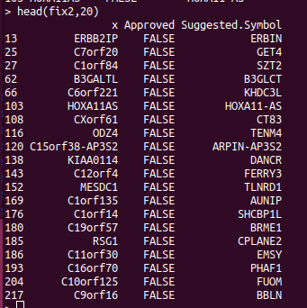
If you are doing analysis of microarray data such as Infinium methylation arrays, then those genomic annotations you're using might be several years old.  The EPIC methylation chip was released in 2016 and the R bioconductor annotation set hasn't been updated much since. So we expect that some gene names have changed, which will reduce the performance of the downstream pathway analysis. The gene symbols you're using can be updated using the HGNChelper R package on CRAN. Let's say we want to make a table that maps probe IDs to gene names, the following code can be used. library("IlluminaHumanMethylationEPICanno.ilm10b4.hg19") anno <- getAnnotation(IlluminaHumanMethylationEPICanno.ilm10b4.hg19) myann <- data.frame(anno[,c("UCSC_RefGene_Name","UCSC_RefGene_Group","Islands_Name","Relation_to_Island")]) gp <- myann[,"UCSC_RefGene_Name",drop=FALSE] gp2 <- strsplit(gp$UCSC_RefGene_Name,";") names

It has been an amazing year of research. I've been at Burnet Institute since August 2023 as Head of Bioinformatics and I've really enjoyed the challenge of serving the many and varied 'omics projects at the Institute and loved discussing new project ideas with everyone here. I'm still active at Deakin in student supervision and project collaborations and this is ongoing. In terms of research directions, my group has been focused on our three themes:  1. Bioinformatics collaborative analysis 2. Building better software tools for omics analysis 3. Reproducibility and research rigour Some of the long-running projects have been completed including methylation analysis of type-1 diabetes complications, which has been about 10 years in the making [1]. The number of collaborative projects has dipped, which is normal when changing institutes and I hope this will lift in the coming years as Burnet work gets completed. In terms of research directions for 2024, there are many. One

There have been a few papers recently on “green computing”, and changes we can make to ensure our work is more sustainable. The most important aspect to this is the overuse of energy in conducting our analysis, especially if the energy is derived from burning fossil fuels. What I want to do here is to put in context the energy expenditure of research computing systems by comparing it to other energy expenditures such as travel and transport. Energy consumption of a workstation or small server In order to quantify the energy expenditure of a compute system, we need to make some assumptions. We will assume that for bioinformatics, the CPU is the main consumer of power, is working at 50% of capacity. AMD Ryzen 9 5950X (16 cores / 32 threads) Maximum power consumption = 142 W /2 = 71 W source High end motherboard: 75 W. RAM stick: 3 W * 8 = 24 W Mid range graphics card idle = 12 W HDD Storage: 9 W * 2 = 18 W Total: 71 + 75 + 24 + 12 + 18 = 200 W So a workstation, or small server with 32 th

I’ve been thinking a lot about best practices lately. I even co-wrote a best practices article just last month. As I have been working with students and colleagues and reflecting on my own practices I have come to the conclusion that us researchers need to align our work more closely towards software developers rather than other researchers. In software development there is a strong differentiation between “development” and “production” work environments. Production is the live app after release to consumers, it is critical that the app functions as expaected, is reliable, useful and with a good user experience. This is after all, where these tech companies make their money. Any downtime is going to be embarrassing and will cost the company money and customers. The development environment on the other hand is the place where software developers can experiment with creating new features, prototype, and refine ideas. As things are built, the software code contains lots of bugs, and this

I've been working on a new project to follow-up our paper last year on the problems with pathway enrichment analysis.  That article turned out to be a bleak and depressing look into how frequently used tools in genomics are misused. It is not an exaggeration to say that most articles showing some type of enrichment analysis are doing it wrong and no doubt this is severely impacting the literature. However I think it isn't helpful to only focus on the negative aspects of bioinformatics and computational research. We also need to lead the way towards resolving these issues. The best way to do this is in my view is to provide step-by-step guides and tutorials for common routines. So this is what we are in the process of doing, making a protocol for pathway enrichment analysis that is "extremely reproducible". By this, I mean that the analysis could be reproduced independently in future with the minimum of fuss and time. As we were writing this we also recognised that the

Also called kernel density plots, these are two-dimensional contour heatmaps which are useful to replace scatterplots when the number of datapoints is so large that it risks overplotting. I've used these sort of plots for many years, most notably in the mitch bioconductor package where it is used to map the relationship of differential expression between two contrasts. There are solutions in ggplot, but I thought I'd begin with a base R approach. In the example below, some random data is generated and plotted. Just subsitute your own data and give it a try.     xvals <- rnorm(100,10,100) yvals <- rnorm(100,10,200) mx <- cbind(xvals,yvals) palette <- colorRampPalette(c("white", "yellow", "orange", "red",   "darkred", "black")) k <- MASS::kde2d(mx[,1], mx[,2]) X_AXIS = "x axis label"                              Y_AXIS = "y axis label"                              filled.contour(k, co

Performing a differential methylation analysis of infinium array data requires an impressively large number of R packages, such as `minfi`, `missmethyl`, `limma`, `genomicRanges`, `DMRcate`, `bunpHunter` and many others. Each of these in turn are considered heavy packages as they each require many dependancies. This means it can take up to an hour to go from a vanilla R installation to one with all the needed packages installed. If you are using multiple computers you might find that these have slightly different versions of R, bioconductor and this large stack of dependancies, which could lead to different results. You may also find that it is difficult to install this large set of dependancies on shared systems, as some dependenncies might require installation of system libraries that need admin permissions to install. The way I've tried to alleviate this problem is to install all my needed packages into a Docker image which can then be downloaded and run in a few minutes on a ne