Comparing expression profiles

One of the most common tasks in gene expression analysis is to compare different profiling experiments. There are three main strategies:

1. Compare all data points - using a correlation analysis
2. Compare sets of up and down-regulated genes - using a binomial or Fisher exact test
3. Compare sets of genes within a profile - such as GSEA test

In this post, I'll describe how correlation analysis is used between expression data sets of all detected genes.

Merging data sets

No matter what type of correlation used, the profiling data sets need to be merged. This means selecting a field that can the datasets can be merged on. This could be a array probe ID, gene accession number or gene symbol as in this case. I will compare gene expression profiles from two experiments (azacitidine in human and mouse cells). The human gene profile was generated by RNA-seq and the mouse data set by microarray.

The human data is currently in CSV format from Degust  and looks like this:

gene,c,aza,FDR,C1,C2,C3,A1,A2,A3
LYZ,0,-1.65809730597384,4.70051409587021e-16,17393,14675,16300,4951,5064,4841
IFI27,0,-3.40698193025161,1.01987358298544e-15,5695,5552,4630,475,532,442
SLC12A3,0,-3.46002052417193,6.78905193176251e-14,1129,1051,991,79,109,92
HLA-B,0,-1.41354726616356,6.78905193176251e-14,6678,5597,5567,2167,2281,2042

The mouse gene symbols were converted to human as per a previous post and look like this:

MusGeneSymbol MouseAccession HumanAccession HumanGeneSymbol FoldChange P-value adjP-value
Krt8 ENSMUSG00000049382 ENSG00000170421 KRT8 6.9755573 2.24e-08 0.000346
Rpl39l ENSMUSG00000039209 ENSG00000163923 RPL39L 3.8096523 2.32e-08 0.000346
Sprr1a ENSMUSG00000050359 ENSG00000169469 SPRR1B -3.441516 6.46e-08 0.000378
Sprr1a ENSMUSG00000050359 ENSG00000169474 SPRR1A -3.441516 6.46e-08 0.000378





So here's a way to perform the join in the UNIX shell environment:

#first sort the mouse spreadsheet on the field to be 
#joined (human gene symbol)
sort -k 4b,4 mouse.xls > mouse_s.xls

#manipulate the human expression data
#remove header, convert to tabular file then sort
#on gene symbol and join with the mouse file
sed 1d human.csv | tr ',' '\t' | sort -k 1b,1 \
| join -1 1 -2 4 - mouse_s.xls > human+mouse.xls

Now have a look at the number of lines in the files, there will be fewer genes that were detected in both experiments, in this case, just 10914 genes for comparison.

  15586 human.csv
  16421 mouse.xls
  10914 human+mouse.xls

Pearson correlation based on fold change

This is perhaps the most simple analysis of two datasets could be done based on similarities of the expression fold changes.

#Open an R session
#load in the data
x<-read.table("human+mouse.xls")
pdf(file="foldchanges.pdf")
#plot the mouse fold change (col 14) against 
#the human fold change (col3)
plot(x$V14,x$V3, xlab="mouse", ylab="human")
dev.off()

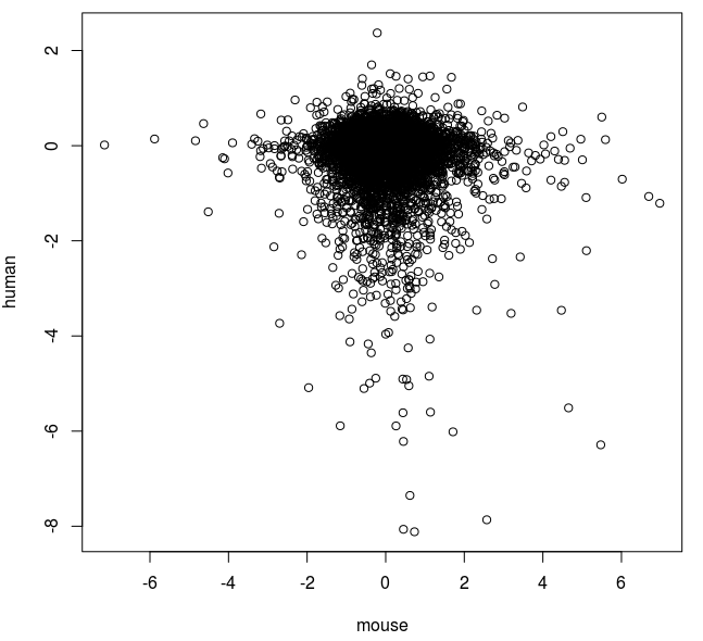Comparison of fold changes in mouse and human cells exposed to azacitidine.

If we want to plot the trend line and the Pearson correlation then we can follow the tutorial here.

Comparison of fold changes in mouse and human cells exposed to azacitidine now including trend line equation and correlation coefficient.

So it seems that there is a slight negative correlation with this method. We also see that a relatively few extreme values seem to be influencing the correlation.

Spearman correlation based on fold change

The Spearman correlation could be better because it is less susceptible to outliers. We rank the genes from highest fold change to lowest with the R rank command. Once the genes are ranked, use the Pearson procedure above to plot the graph.

#make a new dataframe containing the ranks
y<-data.frame(x$V1, rank(x$V14, na.last = NA , ties.method = c("average")) , rank(x$V3, na.last = NA , ties.method = c("average")))
plot(y$mouse,y$human,cex=.5,xlab="mouse rank", ylab="human rank")
spearmans_r = cor(y$mouse,y$human)
r_squared = spearmans_r^2
fit = lm(y$human~y$mouse)
y_intercept = as.numeric(fit$coeff[1])
slope = as.numeric(fit$coeff[2])
abline(lm(y$human~y$mouse),col="red")
function_string = paste("f(x) = ", slope, "x + ", y_intercept,  sep="")
r_sq_string = paste("R^2 =", r_squared)
display_string = paste(function_string, r_sq_string, sep="\n")
mtext(display_string, side=3, adj=1)

Spearman correlation of fold changes between two expression profiling experiments.

From the graph, we see that apart from a few genes clustered in the corners, overall there is only a very slight negative correlation.

Pearson correlation based on p-value derived differential expression metric 

The fold change might not be the best metric to perform these comparisons because many of the genes with variable fold changes could have high p-values, and hence not be that reliable. The differential expression metric (DEM) I use is the signed log10-transformed p-value with the sign denoting the direction of change, positive for increasing and negative for decreasing (reference). I use the raw (not FDR) p-value because it has a smoother dynamic range. I presented the bash script for generating the DEM in a recent post. I used that script to generate DEM scores for each experiment then joined them as above.

Pearson correlation of differential expression metric (DEM) scored derived from p-values.

The result again shows only a very slight negative correlation.

Spearman correlation based on p-value derived differential expression metric

I ranked the genes by DEM score and plotted it.

Spearman correlation of differential expression metric (DEM) scored derived from p-values.

This result shows a vanishingly small negative correlation.

Conclusion

I used four methods to analyse similarity between the expression profiles. Unexpectedly, the four analyses all showed that azacitidine treatment produced quite different results in these two contexts. That could be due to factors such as the difference in cell type used (human AML3 vs mouse C2C12), the profiling platform (human by RNA-seq and mouse by array) or other factor.